


3.2 Mapping
We can use self-organizing maps to lower the dimensionality and preserve the topological features of the data. To complete this task, we present to the input layer the distance vectors, i.e. the coordinates of each resource as a point in an  -dimensional space,
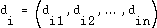 .
.
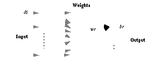
The neurons in the competitive layer are in fact the pixels  and a weight (reference) vector
  is associated with them:
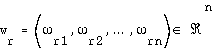
with  .
.
 |
The self-organizing map algorithm in the learning process stage[7] can be summarized as follow:
 and a weight vector
  of the neuron
  :
: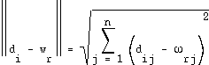
 is defined as the one which has the closest weight vector:
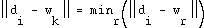
During the learning period, a neighborhood function  is defined to activate neurons that are topographically close to the winning neuron. This function is usually
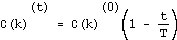
where  is the initial neighborhood (radius)[9].
The reference vectors of the neurons surrounding the winner are modified as follows: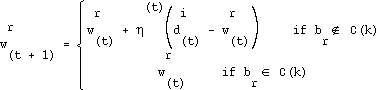
with  a monotonically decreasing function, for example:
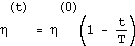
 being the initial learning rate[10] and
  the number of training operations.[11]
Note that self-organizing maps are performed in a way similar to the k-means [Belaïd and Belaïd, 1992] algorithm used in statistics. Although, the latter has been shown to perform differently and less satisfactory than the first [Ultsch, 1995]
It must be noted that no proof of convergence of the self-organizing maps algorithm, except for the one-dimensional case, has yet been presented [Kohonen, 1995]. Although, it is important to evaluate the complexity of the algorithm. Since the convergence has not be formally proved, we must rely on empirical experiments to determine  . Thus, for
  , it has been shown that the complexity of the algorithm is of the order
  [Wyler, 1994].
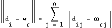
Having completed the learning process, the mapping can be processed by calculating for each input distance vector the winning neuron. We have then a mapping function which for each resource  returns a pixel
  :
: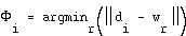 .
.
 .
.
 should be at least 500
 during the final convergence phase.